Three panels, each requestable via which:
- 1
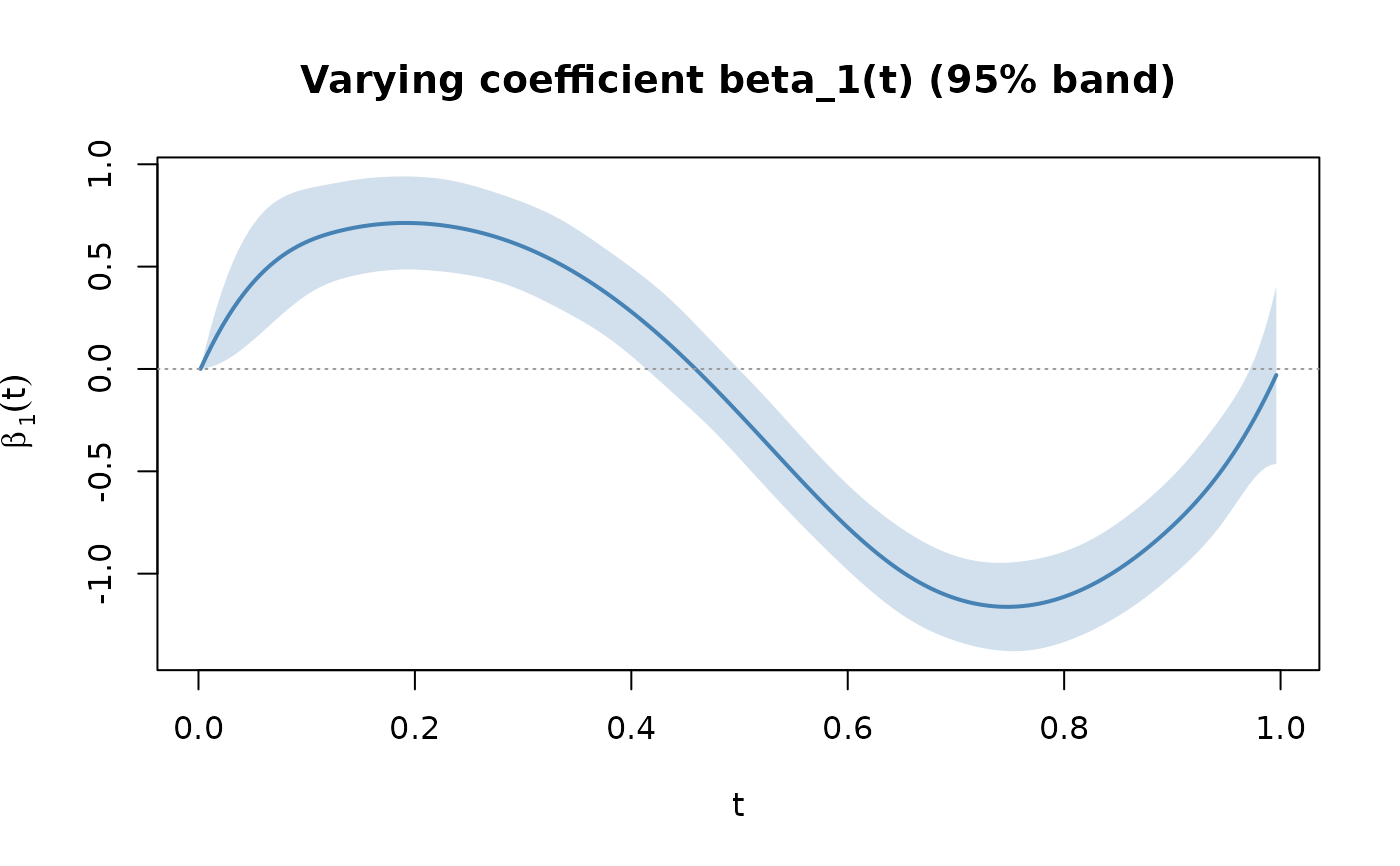
Varying-coefficient curves \(\hat\beta_k(t)\) with pointwise Wald confidence bands.
- 2
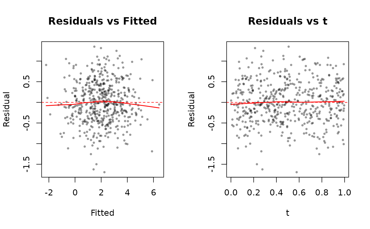
Residual diagnostics: residuals vs fitted, residuals vs \(t\). Requires
datasince a vcmm fit does not carry the raw training data.- 3
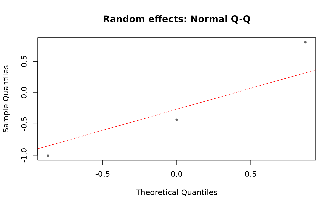
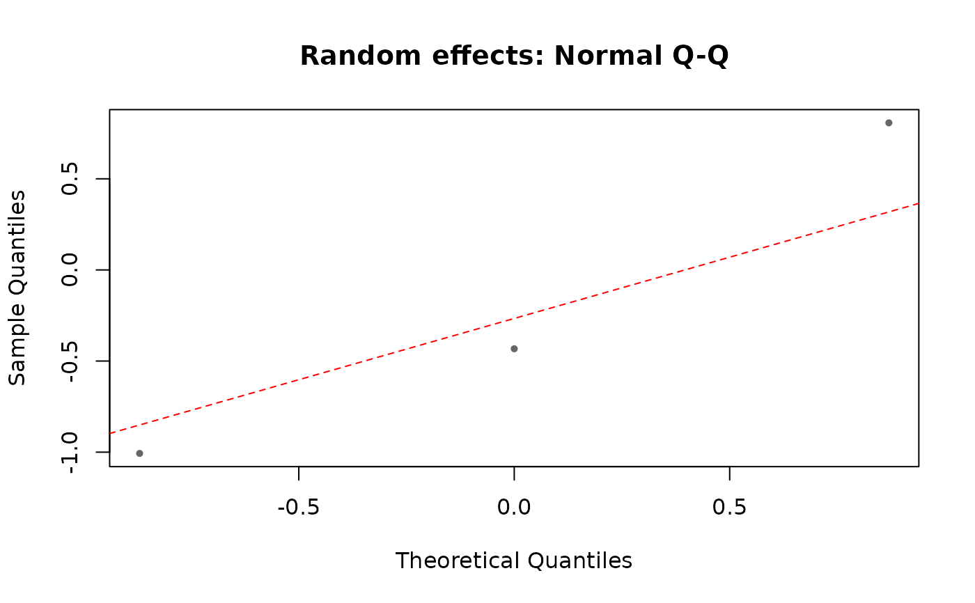
Random-effects diagnostics: Normal Q-Q for
re_cov = "diag", or a heatmap of the \(G \times q_{\mathrm{left}}\) random-effects matrix together with a heatmap of the estimated \(\Sigma_{\mathrm{left}}\) for"kronecker"/"separable".
Usage
# S3 method for class 'vcmm_fit'
plot(
  x,
  which = 1:3,
  data = NULL,
  t_grid = NULL,
  n_grid = 200L,
  conf_level = 0.95,
  ask = (length(which) > 1L) && interactive(),
  ...
)
Arguments
- x
A
vcmm_fitobject.- which
Integer vector subset of
1:3. Default1:3.- data
Optional list with components
y,X,Z,t(the training data, or any data on which to compute residuals). Required when panel 2 is requested.- t_grid
Numeric. Grid of \(t\) values for panel 1. Default
NULLmeans an evenly-spaced grid over the stored training range[t_min, t_max].- n_grid
Integer. Number of grid points if
t_gridisNULL. Default 200.- conf_level
Numeric in (0, 1). Confidence level for panel-1 bands. Default 0.95.
- ask
Logical. Passed to
devAskNewPage()when multiple panels are requested in an interactive session.- ...
Further arguments passed to base graphics calls.
Details
Uses base R graphics, no ggplot2 dependency. Each requested
panel is drawn on its own figure (or set of subfigures via
par(mfrow)); call par(mfrow = c(2, 2)) or similar
before plot() to combine panels in one figure.
References
Jalili, L. and Lin, L.-H. (2025). Scalable and Communication-Efficient Varying Coefficient Mixed-Effects Models.
Examples
set.seed(1)
n <- 500
t <- runif(n); x <- runif(n); Z <- matrix(rnorm(n * 3), n, 3)
a <- rnorm(3, sd = 0.5)
y <- 2 + sin(2 * pi * t) * x + as.vector(Z %*% a) + rnorm(n, sd = 0.5)
fit <- vcmm(y, X = x, Z = Z, t = t,
control = vcmm_control(sigma_eps = 0.5, sigma_alpha = 0.5))
# \donttest{
plot(fit) # all three panels
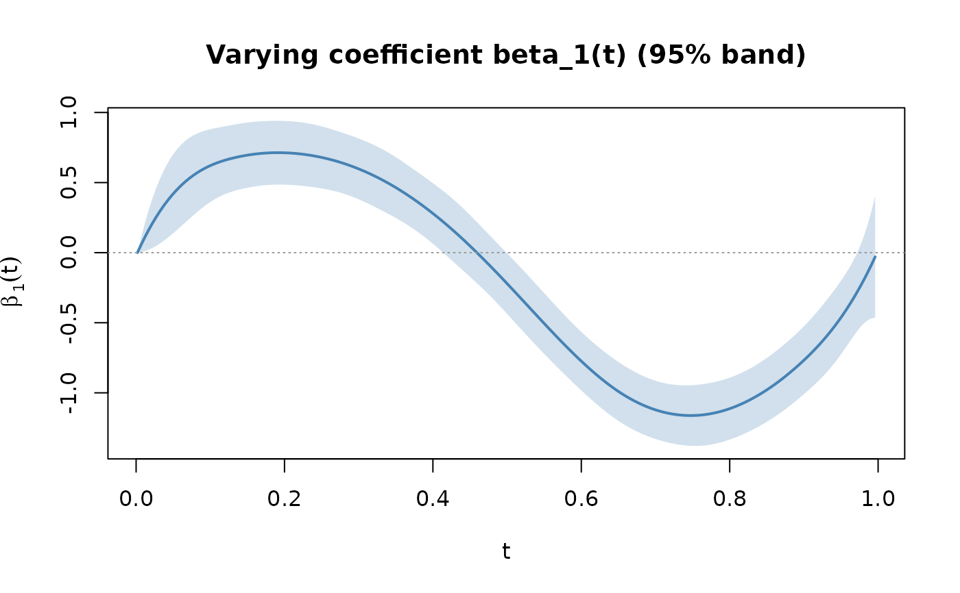 #> Warning: plot.vcmm_fit: panel 2 requires `data` (a list with y, X, Z, t). Skipping.
 plot(fit, which = 1) # only varying coefs
 plot(fit, which = 2, data = list(y = y, X = x, Z = Z, t = t))
 plot(fit, which = 3) # ranef diagnostics
 # }
# }